The crux with reducing emissions in the long-term: The underestimated “now” versus the overestimated “then”
Abstract
The focus of this perspective piece is on memory, persistence, and explainable outreach of forced systems, with greenhouse gas (GHG) emissions into the atmosphere serving as our case in point. In the light of the continued increase in emissions globally vis-à-vis the reductions required without further delay until 2050 and beyond, we conjecture that, being ignorant of memory and persistence, we may underestimate the “inertia” with which global GHG emissions will continue on their increasing path beyond today, thus, also leading to the amount of reduction that can be achieved in the future being overestimated. This issue is at the heart of mitigation and adaptation. For a practitioner, this translates to the problem of how persistently an emissions system behaves when subjected to a specified mitigation measure and which emissions level to adapt to for precautionary reasons in the presence of uncertainty. Memory allows us to reference how strongly the past can influence the “near-term future” of the system or (what we define as) its explainable outreach. We consider memory to be an intrinsic property of a system, retrospective in nature; and persistence to be a consequential (i.e., observable) feature of memory, prospective in nature and reflecting the tendency of a system to preserve a current state (including trend). Persistence depends on the system’s memory which, in turn, reflects how many historical states directly influence the current one. The nature of this influence can range from purely deterministic to purely stochastic. Different approaches exist to capture memory. We capture memory generically with the help of three characteristics: its temporal extent and both its weight and quality over time. The extent of memory quantifies how many historical data directly influence the current data point. The weight of memory describes the strength of this influence (fading of memory), while the quality of memory steers how well we know the latter (blurring of memory). Capturing fading and blurring of memory in combination is novel. In a numerical experiment with the focus on systemic insight, we cast a glance far ahead by illustrating one way to capture memory, and to understand how persistence plays out and how an explainable outreach of the system can be derived even under unfavorable conditions. We look into the following two questions: (1) Do we learn properly from the past? That is, do we have the right science in place to understand and treat memory appropriately? And (2) being aware that memory links a system’s past with its near-term future, do we quantify this outreach in a way that is useful for prognostic modelers and decision-makers? The latter question implies another question, namely, whether we can differentiate between and specify the various characteristics of memory (i.e., those mentioned above) by way of diagnostic data-processing alone? Or, in other words, how much system understanding do we need to have and to inject into the data-analysis process to enable such differentiation? Although the prime intention of our perspective piece is to study memory, persistence, and explainable outreach of forced systems and, thus, to expand on the usefulness of GHG emission inventories, our insights indicate the high chance of our conjecture proving true: being ignorant of memory and persistence, we underestimate, probably considerably, the “inertia” with which global GHG emissions will continue on their historical path beyond today and thus overestimate the amount of reductions that we might achieve in the future.
Keywords
Earth system science Greenhouse gas Emissions inventory Data analysis Memory Persistence Explainable outreach Uncertainty1 Introduction
This article is a perspective piece on research still to be conducted and elaborated in scientific papers. Its focus is on forced systems exhibiting memory, with greenhouse gas [GHG] emissions into the atmosphere serving as an example. Here, we ask two simple questions: (1) Do we learn properly from the past? And (2) being aware that memory allows us to reference how strongly a system’s past can influence its near-term future, do we quantify this “outreach” in a way that is useful for prognostic modelers and decision-makers?
The answer to both questions is no, as we argue below, the reason being that we do not have the right science in place to address these questions adequately. Embarking on such research will lead us to new grounds needing to be mapped and explored—which is why we opt for a perspective piece before anything else. We are lacking tools to fully understand the nature of memory in systems and its effect. As a first consequence, the questions lead us to the need to fuse deterministic and statistical data analysis to complement process modeling (question 1) and to the need to establish (what we call) the explainable outreach [EO] of data series with memory (question 2).
As a further consequence, the two questions together point to an important, widely observed problem: we typically underestimate the tendency of systems with memory to continue on their historical path into the future. In the case of GHG emissions, we face the need to reduce emissions instantaneously. Being ignorant of memory and persistence, a consequential feature of memory, we underestimate—most likely, even considerably—the tendency with which GHG emissions, currently still increasing globally (Carbon Brief 2017), will continue on their historical path beyond today; and thus we overestimate the amount of reductions that we can achieve in the near future. This issue is at the heart of mitigation and adaptation. For a practitioner, it translates to the problem of how persistent an emissions system's behavior is when it is subjected to a specified mitigation measure and which emissions level to adapt to for precautionary reasons in the presence of uncertainty.
Although GHG emissions, notably CO2, into the atmosphere serve as our prime real-world example, we gain a more fundamental understanding of the problem by initially working under lab conditions, i.e., with synthetic data (as done here). Nonetheless, any other series of data (observations) of systems with memory, e.g., atmospheric CO2 concentrations or average surface air temperature changes, can also be used, preferably in combination.
2 Motivating a broader perspective of memory
It is in the context of analyzing the structural dependencies in the stochastic component of time series where the terms “memory” and “persistence” commonly appear and are widely discussed.
However, we start from an accurate and precise world where we observe memory (precisely). In this world, time series analysis, being statistically grounded, is inappropriate for deal with memory (noise does not exist). This must be done differently. Only then do we make the step, common in physics, to an accurate and imprecise world, the realm of time series analysis.
Our intention in defining memory independently (i.e., outside) of time series analysis is not to exclude time series analysis, but to explore (1) how memory defined in an accurate and precise world “spills over” and impacts time series analysis in an accurate and imprecise world and (2) the advantage of treating memory (more specifically, its characteristics) consistently for both the deterministic and the stochastic part of a time series.
In the further course of the perspective piece, we will encounter additional advantages that will justify this two-pronged approach. These include not being restricted to working with small numbers which are, not unusually, also in the noise range (a consequence of making time series stationary); and being able to introduce gradual blurring of memory (increase in uncertainty back in time) as the unavoidable twin effect accompanying the fading of memory (decrease in memory back in time). To our knowledge, these two memory characteristics have not been addressed in combination to date.
Above and beyond, there is another fundamental difference to time series analysis: We do not attempt to predict. Instead, we make use of the memory characteristics of a time series to determine its explainable outreach [EO] (as visualized in Section 4 and demonstrated in Section 6).
2.1 Motivating by way of example
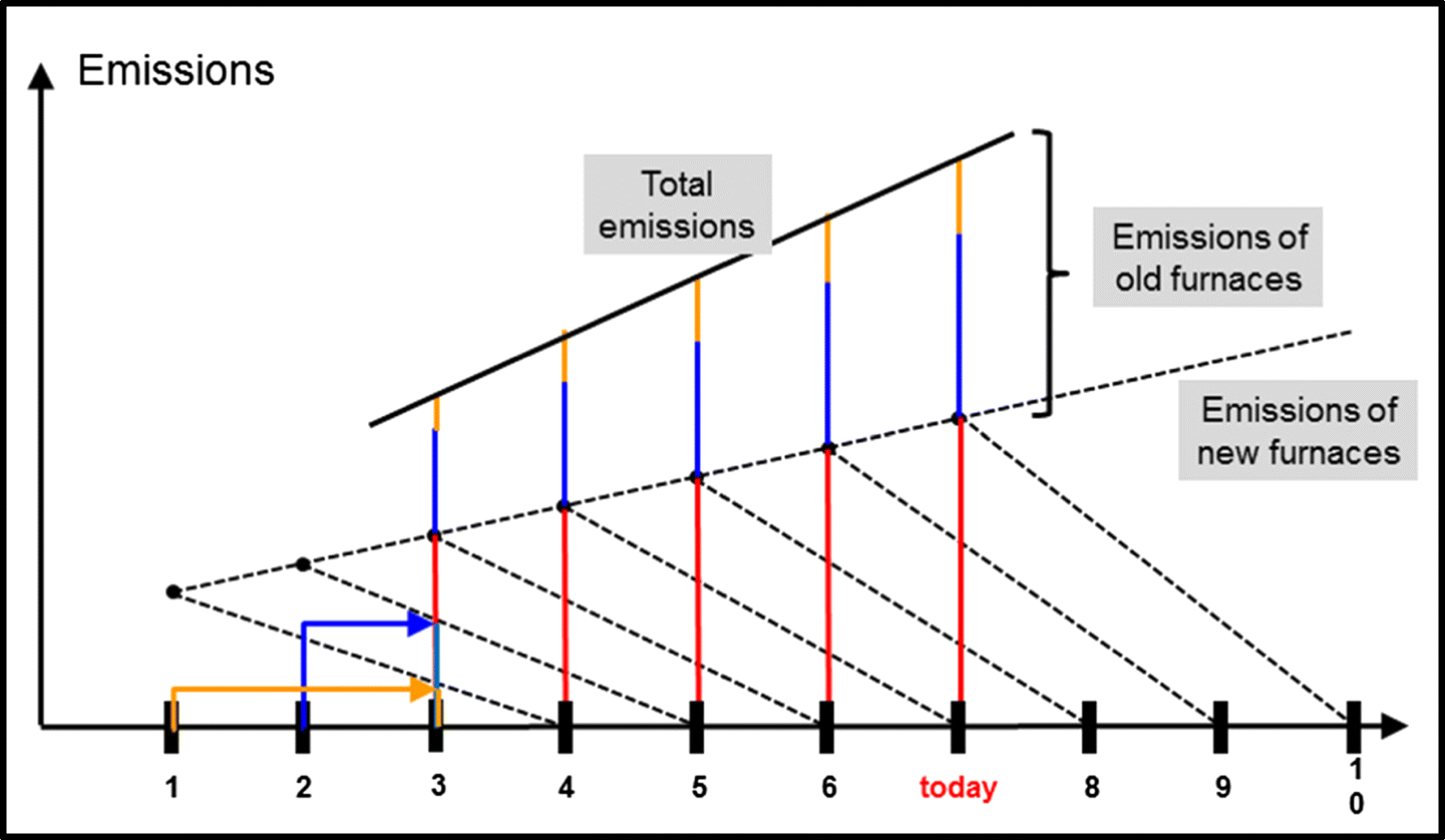
Example illustrating the memory effect: old furnaces still contribute to emissions accounted today. Horizontal axis: time; vertical axis: emissions. Conditions are assumed constant for a given time; this means that, during that time, furnaces phase in instantaneously (here at a linearly increasing rate) and phase out linearly (here over 3 years). Red: emissions of newly installed furnaces at any current point in time; blue: emissions of 1-year-old furnaces contributing to current emissions (added on top of the red bars); orange: emissions of 2-year-old furnaces contributing to current emissions (added on top of the red-blue bars). Total emissions are given by the red-blue-orange bars
It can be argued that emissions from newly installed furnaces as well as total emissions are better known than emissions from older furnaces. On the one hand, countries that make estimates of CO2 emissions under the UNFCCC (United Nations Framework Convention on Climate Change) provide annual updates in which they add another year of data to the time series and revise the estimates for earlier years (bottom-up approach) (Marland et al. 2009; Hamal 2010; UNFCCC 2018). On the other hand, high-resolution carbon-observing satellites are able to provide emission accounts (top-down approach) (e.g., Oda et al. 2018), such as the Japanese Greenhouse Gases Observing Satellite [GOSAT] (Matsunaga and Maksyutov 2018) and NASA’s Orbiting Carbon Observatory-2 [OCO-2] (Hakkarainen et al. 2016).
This suggests that our starting point, Fig. 1, should be modified, as follows: At each point in time, we assume that we are able to “measure” precisely both CO2 emissions from newly installed furnaces and total CO2 emissions (which corresponds to knowing the red and the red-blue-orange bars in Fig. 1).
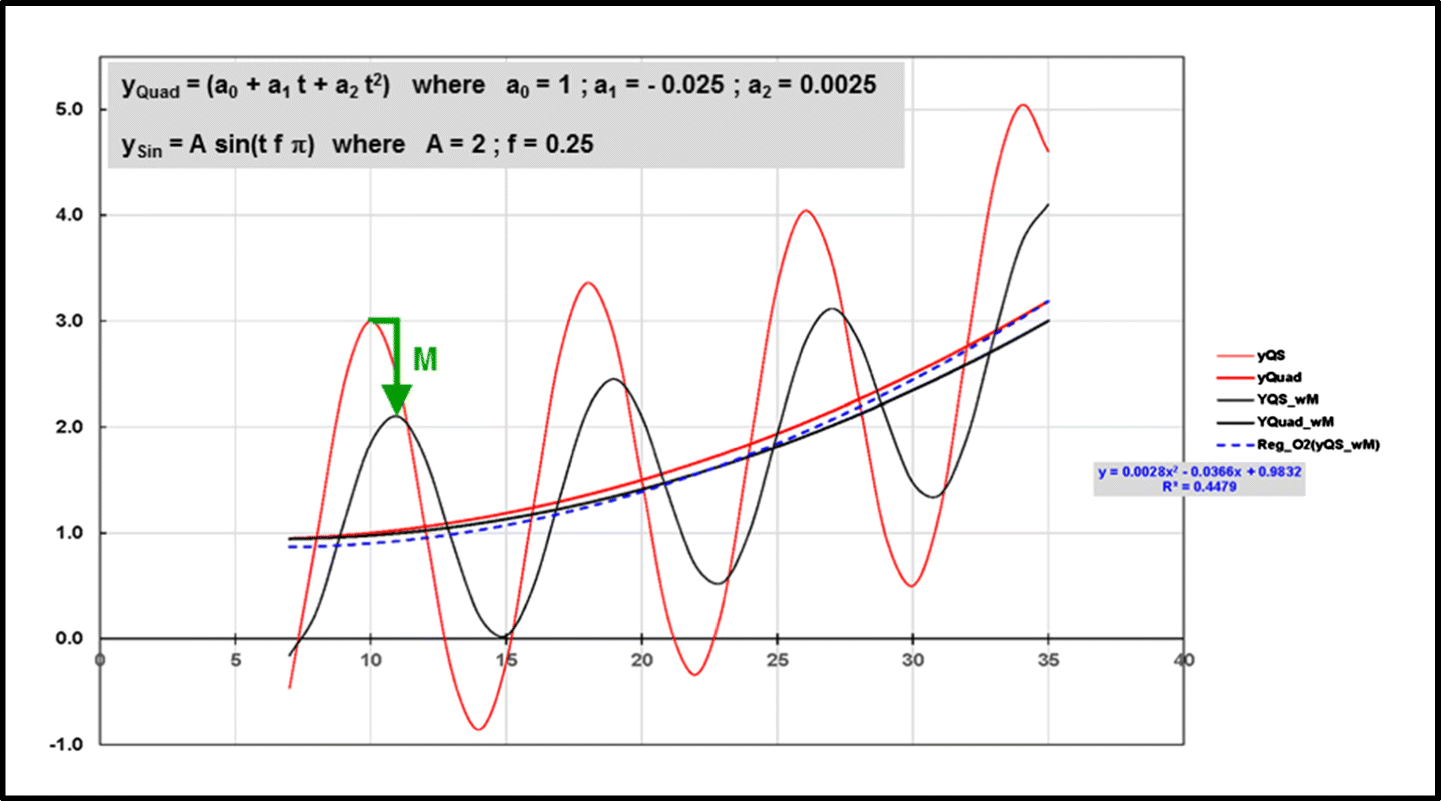
Example shown in Fig. 1 modified. World without memory (no distinct index): given by emissions from newly installed furnaces (yQS ≔ yQuad + ySin; red). World with memory [wM]: given by total emissions (yQS _ wM ≔ yQuad _ wM + ySin _ wM; black). Horizontal axis: time; vertical axis: emissions. Note that both yQS and yQS _ wM describe hypothetical emissions (not shown for the first 7 years, the phase-in time of the moving average) and are normalized (their emissions are 1 at t = 0). Applying a simple moving average to yQS—equivalent to conceiving the application of the memory model M as convolution—allows the transition to yQS _ wM. The second-order regression of yQS _ wM (Reg _ O2(yQS _ wM); dashed blue curve) smoothes yQS _ wM but does not capture its true trend yQuad _ wM (=yQuad∗M). The same holds for the second-order regression of yQS (not shown)
Additional information to Fig. 2
The example shows that determining M can/should happen outside of time series analysis (e.g., by way of deconvolution). Knowing M is also key in determining the true trend of yQS _ wM (i.e., yQuad _ wM). In further consequence, yQS _ wM cannot/not easily be detrended correctly (see Reg _ O2(yQS _ wM) in Fig. 2) if M is unknown. But correct detrending is tacitly presupposed in making time series stationary.
2.2 Motivating more generally
As mentioned, our focus is on systems with memory, typical in Earth system sciences. In addition, we restrict ourselves to forced systems. In many cases, we do know that a system possesses memory, e.g., because it does not respond instantaneously to the forcing it experiences—which is what a system with no memory would do. (This becomes visible in Fig. 2: yQuad _ wM lags behind yQuad.)
Such systems are typically dealt with by using one of two approaches: (1) process-based modeling (e.g., Solomon et al. 2010) and (2) time series analysis (e.g., Belbute et al. 2017). With reference to our example, the first approach would be equivalent to modeling the stock, i.e., the phase-in and phase-out, of furnaces over time; the second approach would be equivalent to subtracting trend and (ideally) periodicity from a time series to determine the dependency structures in the random residuals.
Each approach comes with strengths and weaknesses. The first approach is useful in gaining systemic insight and understanding of, how a system responds to an applied forcing and close to or beyond systemically important thresholds. However, this approach typically goes hand-in-hand with an increased need for data and may fall short of describing reality correctly (thus, also projections into the future). By way of comparison, the second approach is purely data-driven. Its strength lies in interpreting a data series statistically, i.e., without seeking to understand (at least, not primarily) the processes impacting and governing the system. However, this approach requires correct detrending; dealing, as a result of this, with potentially small numbers; and addressing the challenge of reflecting the statistical properties of (what time series analysts call) the data-generating process underlying the series’ residuals.
Of course, this data-generating process also leaves its mark on the deterministic part of the series. But this is simply not considered or overlooked. Take memory as an example. Testing the residual of a time series for stationarity does not imply that we capture the influence of M on the deterministic part of the time series. This can easily be shown with the help of our example (cf. Figures 2 and 1): Change the trend of yQS from nonlinear back to linear, omit periodicity but add white noise instead; and then apply a simple moving average (our memory model M)—which will not change the linear trend per se. That is, in making the time series stationary, a linear trend is subtracted from the time series without awareness being created that the trend had been impacted by memory. We recall that the situation is more challenging in the case where yQS _ wM exhibits a nonlinear trend. Correct detrending is then not/not easily possible any longer unless M is known. In general, it can be said that the two-pronged characterization of systems in terms of trend and fluctuations around that trend is widely recognized (e.g., Kantelhardt 2004), but memory is not understood as an important element connecting the two.
Hence, the question (referred to as question 1 above) arises as to how to treat memory (more specifically, its characteristics) consistently across both the deterministic and the stochastic part of a time series? This question needs to be addressed by applying a deterministic-stochastic approach, initially under controlled (i.e., lab) conditions. This approach would contribute to filling the aforementioned gap in science and can be considered as falling in between process-based modeling and time series analysis.
2.2.1 From an accurate and precise world
When we speak of memory in a deterministic context, we refer to the momentum of a system over “some” historical time range. In the physical world of Newtonian systems, momentum indicates a system’s inertia. If the momentum is not constant, this indicates how much the system deviates from an inert state due to an external force. Likewise, systems with memory also exhibit inertia, called persistence below. (For inertia in the climate system, refer to, e.g., IPCC 2001: SPM: Q5.)
2.2.2 …to an accurate and imprecise world
There are different approaches to capturing memory. We capture memory generically with the help of three characteristics: its temporal extent, and both its weight and quality over time (see Sections 5 and 6). The extent of memory quantifies how many historical data directly influence the current data point. The weight of memory describes the strength of this influence (fading of memory), while the quality of memory steers how well we know the latter (blurring of memory). Capturing fading and blurring of memory in combination is novel.
Memory allows us to refer to how strongly a system’s past can influence its near-term future. This is by virtue of persistence, the counterpart to memory which, just like momentum, is not to be confused with prediction. The question of interest to us (referred to as question 2 above) is how well we need to know the various characteristics of memory (e.g., the ones mentioned above) in order to delineate a system’s near-term future, which we do by means of (what we call) the system’s explainable outreach [EO] Or, put differently, how much system understanding do we need to have and to inject into the data analysis process to enable the discrimination of memory characteristics and the quantification of the EO? We have reasons to be optimistic that the system’s EO can be derived under both incomplete knowledge of memory and imperfect understanding of how the system is forced. This we illustrate in Section 6.
It appears striking that it is reality—here we refer to the need to reduce GHG emissions instantaneously—which underscores the need to research these two questions: Being ignorant of memory and persistence, we may underestimate, even considerably, the “inertia” with which global GHG emissions will continue on their ever-increasing path beyond today and thus overestimate the amount of reductions that we can achieve in the near future.
3 Literature review
Prior to approaching memory and persistence, it is useful to start by decomposing a time series X(t) = XTrend(t) + S(t)XNoise into a deterministic component XTrend(t), accounting for all systematic or deterministic processes, and a stochastic component S(t)XNoise, consisting of stationary noise XNoise(t) and a scaling function S(t) to describe (e.g., climate) variability (Mudelsee 2014: Section 1). In proceeding, we simplify further—it is here where we deviate from time series analysis—by assuming that memory acts like a linear filter allowing the impact of memory on the two components to be evaluated separately; likewise, persistence as a consequential feature of memory, resulting from the system’s dynamics (e.g., when its current state is directly influenced by previous states) and/or from the structural stochastic dependencies in the observed process.
However, in capturing the deterministic component, memory effects are typically not the main concern. This component is usually described without identifying memory, e.g., by means of suitable regression methods (e.g., linear/polynomial or non-parametric), or through an equation which is supposed to reflect the system’s dynamics and whose parameters are estimated from the data (so-called data assimilation techniques, e.g., Abarbanel 2013). It is usually in models where memory is captured explicitly, e.g., by introducing time delays in response to an applied forcing. Common to all approaches is that they consider the stochastic component as white noise, thereby ignoring its structural dependencies.
Nonetheless, mathematical techniques do exist to deal with memory without being associated with this term explicitly, depending on how memory is realized. For instance, in our example, memory is realized by means of a simple moving average (as a natural first choice), which can also be understood as convolution of a time series containing no memory. Another example is the empirical mode decomposition [EMD] method (Wu et al. 2007), which allows a skillful detrending by perceiving any trend in the data as an intrinsic property of the data but which, to our knowledge, has not yet been applied with the focus on memory.
How memory and persistence are understood and interpreted by various scientific communities
| Field | Terminology | Interpretation | Literature |
|---|---|---|---|
| Climate analysis | Memory, dependence (distinguishing between short-term/short-range and long-term/long-range) | Rate of decay of the autocorrelation function (considered geometrically bounded; but also with exponential, power-rate, or hyperbolic decay) | Caballero et al. (2002), Palma (2007), Franzke (2010), Mudelsee (2014), Lüdecke et al. (2013), Barros et al. (2016), Belbute and Pereira (2017) |
| Also persistence | Long-range memory (also checked by spectral or fluctuation analysis) | ||
| Economy and finance | Serial dependence, serial correlation, memory, dependence | Statistical dependence in terms of the correlation structure with lags (mostly long memory, i.e., with long lags) | Lo (1991), Chow et al. (1995), Barkoulas and Baum (1996), Dajcman (2012), Hansen and Lunde (2014) |
| Also persistence | Positive autocorrelation | ||
| Geophysics and physics | Persistence, dependence, also memory (mostly long-term) | Correlation structure in terms of Hurst exponent or power spectral density; but also system dynamics expressed by regularities and repeated patterns | Majunmdar and Dhar (2001), Kantelhardt et al. (2006), Lennartz and Bunde (2009, 2011) |
The performance of methods to capture memory in the stochastic component (e.g., by means of ARIMA and ARFIMA models) relies on how nonlinear nonstationary data are (pre-) processed, i.e., on how the deterministic component (trend, seasonality, cycles, etc.) is estimated and removed (if need be) in order to obtain, ideally, a stationary series of residuals. In this approach, memory is associated with the structural dependencies in the series’ residuals and not with the deterministic component, which serves only as a means to obtain a (simplified) statistical model to describe the residuals.
However, capturing the deterministic component unskillfully/incorrectly results in artificial structural dependencies in the residuals—which brings us back to our example and the quest for a coordinated approach to treat memory consistently for both the deterministic and the stochastic component. To our knowledge, such a method is not available.
In pursuing a coordinated approach, a number of additional and well-known problems must be expected. For instance, the deterministic component may be overly complex, so that one may be inclined to prefer describing it stochastically. Or the time series may not be long enough to treat long memory unambiguously, causing an apparent trend and thus a dichotomy between the deterministic and stochastic component. This dichotomy is known to several scientific disciplines, e.g., in econometrics, hydrology, and climatology (Mudelsee 2014: Section 4.4). It is (also) for these reasons that we strongly advocate for an approach under controlled lab conditions initially, which would allows us to explore from when on these and other problems begin to become relevant, or whether these problems can be overcome by simple but effective means, e.g., by swapping ignorance for (greater) uncertainty. (This we show in Sections 5 and 6.)
4 Summary of our current understanding of memory, persistence, and explainable outreach
- 1.
We consider memory as an intrinsic property of a system, retrospective in nature; and persistence as a consequential (and observable) feature of memory, prospective in nature. Persistence is understood as reflecting the tendency of a system to preserve a current value or state and depends on the system’s memory which, in turn, reflects how many historical values or states directly influence the current one. The nature of this influence can range from purely deterministic to purely stochastic.
- 2.
Deriving the EO of a data series should not be confused with prediction (nor with perfect forecasting).
- 3.
Figure 3 illustrates the idea of using EOs as a reference for prognostic modelers and decision-makers. We visualize the EO as an uncertainty wedge, which is derived from the historical data of a time series only (applying a mode of learning and testing) and then shifted to its end (= today). Shifting the EO to the end of the series’ historical data has to happen untested and would therefore not be permitted. However, the only reason this forward shift is still done is to provide a bridge into the immediate future, thus a reference for prognostic modelers and decision-makers. Prognostic scenarios falling outside (above or below) the EO, as well as scenarios falling within, but eventually extending beyond the EO, are no longer in accordance with the series’ past—allowing a decision-maker to inquire about the assumptions made in constructing a forward-looking scenario and to interpret these in terms of how effective planned measures (e.g., emission reductions) need to be and/or how long the effectiveness of these measures remains uncertain. Shifting the EO to today requires a conservative systems view which ensures that the system is not exposed to surprises it had not experienced before.
- 4.
Deriving the EO of a data series must not be confused with signal detection. Signal detection requires the time to be determined at which changes in the data series outstrip uncertainty—which is not done here. Take, e.g., the scenario falling above the EO in the figure. The time at which its signal steps out of the uncertainty wedge does not coincide with the temporal extent of the EO.
- 5.
Assuming persistence to be an observable of memory, Fig. 3 would allow persistence to be quantified (not defined). Given its directional positioning, the red-shaded EO in the figure may be described with the help of two parameters, its extent L and its aperture A at the end. We would then say that a data series with a long and narrow EO (the ratio L/A would be great) exhibits a greater persistence than a data series with a short and wide EO (the ratio L/A would be small).
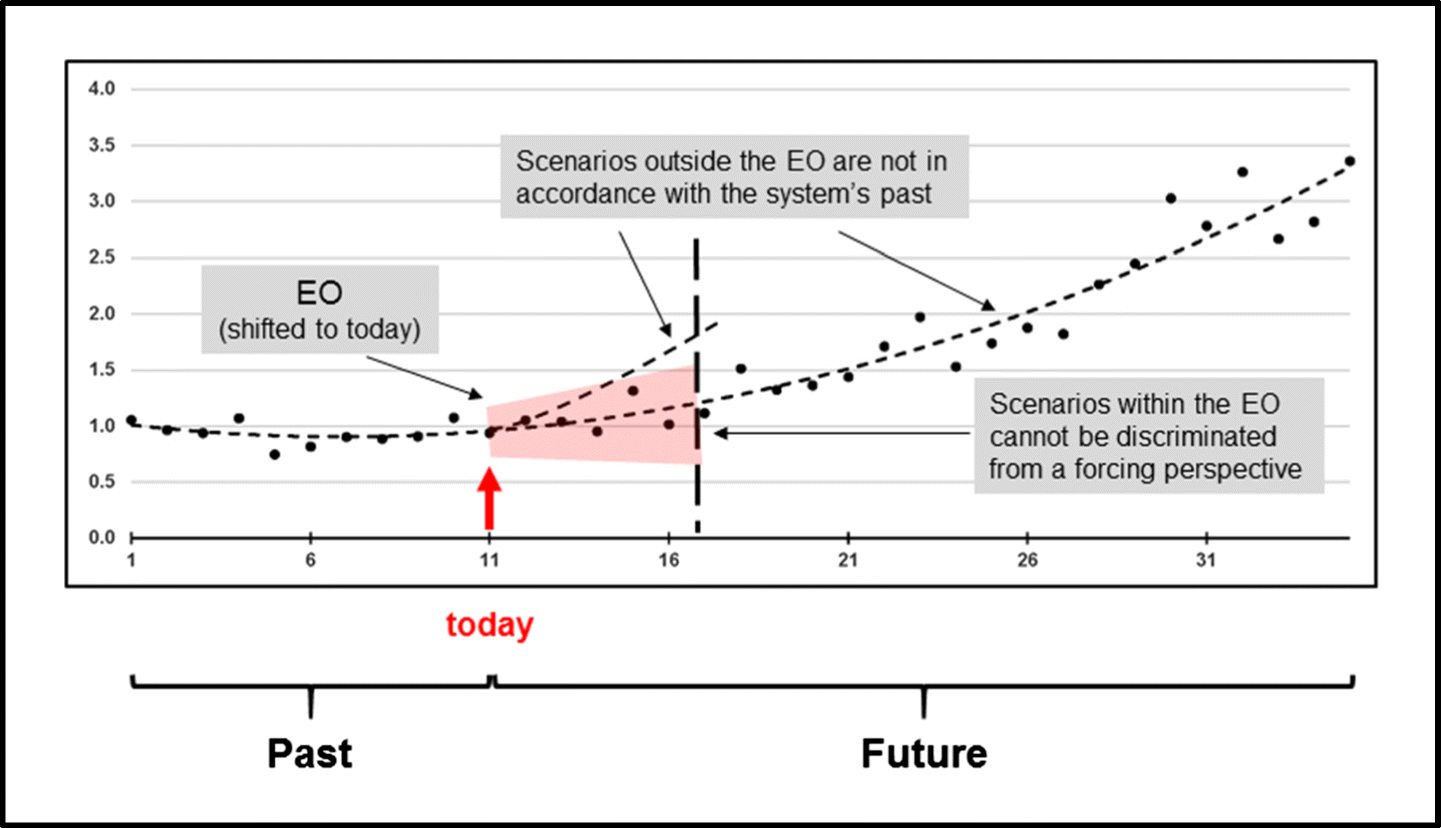
Illustrating why it is important to know the EO of a data series (visualized as an uncertainty wedge; shaded in red). For convenience, in constructing the figure, we assumed a future being known (see black dots in the future part of the data series)
5 Methodology
Our numerical experiment simplifies and extends our example presented in Section 2.1 (trend: preserved; periodicity: omitted; noise: introduced). Mathematical details are mentioned to the extent necessary to keep systemic insight in the focus and to cast a glance far ahead by illustrating one way to capture memory, and also to understand how persistence plays out and how an EO can be derived. We discuss the numerical experiment intensively in Section 7 with respect to how consequential it is, where it underperforms, and the questions it provokes. However, the experiment does not exhibit fundamental shortfalls. It does not restrict generalization, while allowing the important research issues which we will be facing in deriving the EO of a data series to be spotted.
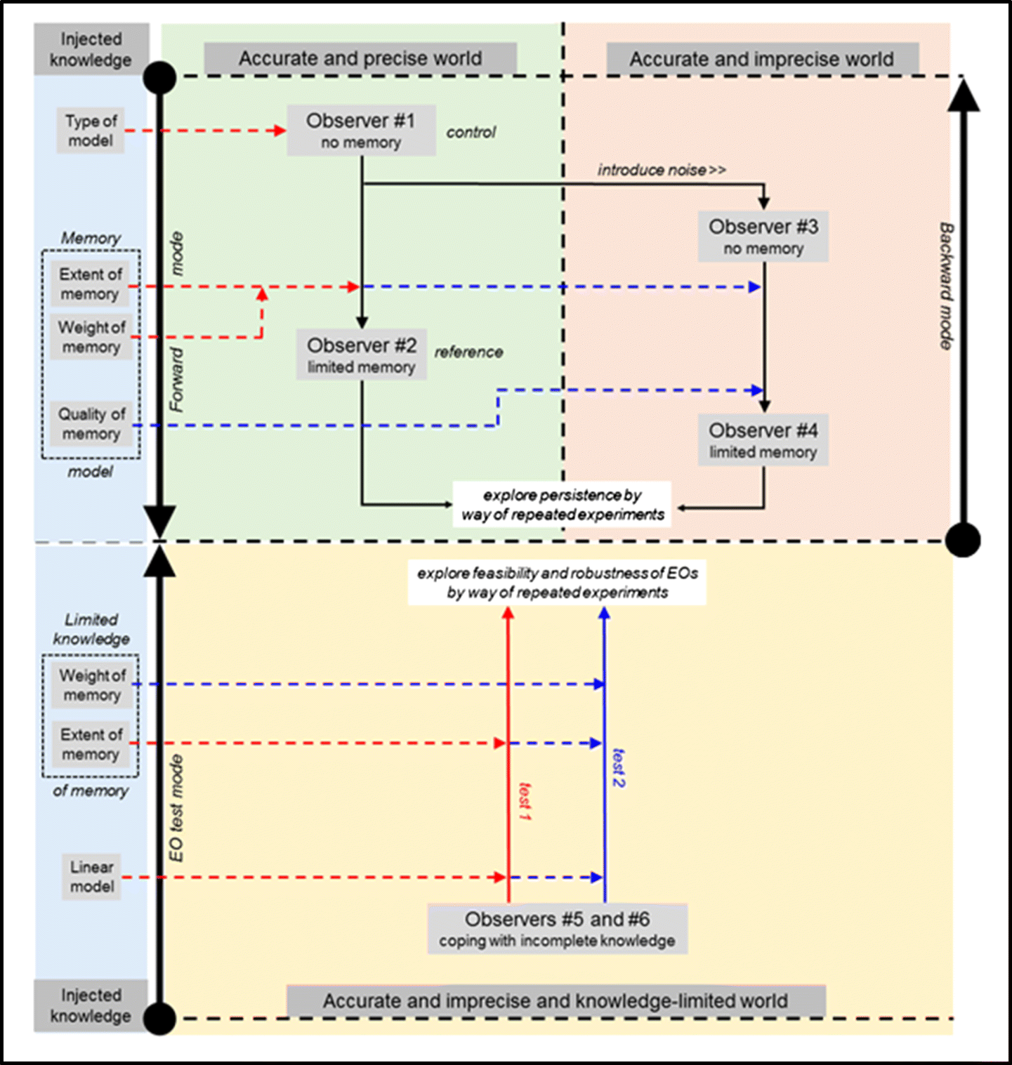
Numerical experiment: graphical visualization of the different “worlds of knowledge.” The figure’s main purpose is to distinguish these worlds based on knowledge that is injected step-by-step (see blue box at the left). Note: The home of the example presented in Section 2.1 is the upper green box
The numerical experiment is composed of two steps. In the first step, we obliterate the knowledge of our control, a second-order polynomial, by applying a high level of noise. In the second step, we offset this obliteration back in time by introducing memory in terms of extent, weight, and quality. This allows the reconstruction, at least partially, of what had been obliterated before. The qualitative and quantitative characteristics of this incomplete reconstruction remain to be investigated against a reference. The intention behind this step-wise procedure is to develop an understanding of how strongly memory plays out and leads to persistence. (Section 6 visualizes this process graphically and also offers a way of deriving an EO.)
We work with four functions dependent on t (with t = 1, ..., 35; sufficiently long for illustration purposes) which can be interpreted as time series with time t measured in years. The functions can be understood as reflecting four observers [O] who perceive an accurate world differently: precisely (O1, O2) or imprecisely (O3, O4); and with perfect knowledge (O1); and limited (O2, O4) or no memory (O3) (see also upper half of Fig. 4). For the sake of simplicity, we drop physical units and proceed dimensionlessly.
All four observers have complete knowledge of their worlds (i.e., t extending from 1 to 35). We introduce two additional observers (O5, O6) later when we split the time series into past (t from 1 to 7) and future (t from 8 to 35). Their knowledge is incomplete because they see the historical part of the time series only (see also lower half of Fig. 4).
5.1 The world of observer O1 is described by
5.2 The world of observer O2 is described by
The notion of memory in connection with yQuad _ wM may not appear straightforward because, ideally, yQuad requires the values of only three points (years) to be entirely determined for all time, all the way from the beginning to the end. On the other hand, we use a memory extent of 7 years when we construct yQuad _ wM with the help of yQuad. Thus, it may be argued that a finite memory becomes meaningless because each individual point of yQuad _ wM carries “full memory.” However, the situation changes if yQuad _ wM is perceived as the extreme outcome of a thought experiment in which the noise surrounding each point of yQuad _ wM decreases to zero eventually.
5.3 The world of observer O3 is described by
In general, we deal with noise in the order of N ≈ 0.10 (that is, N× 100 % ≈ 10%). Here, we increase N by one order, namely to N = 3.0 (that is, N × 100 % = 300%), which may result in YQwN as a whole being perceived as random noise with some directional drift, if at all, rather than a signal that is clearly visible, albeit superimposed by noise.
5.4 The world of observer O4 is described by
To summarize, in introducing memory, we make use of three characteristics: its temporal extent (here dealt with by way of “insightful decision”), and both its weight and quality over time. We show in Section 6 that memory can, but need not, allow partial reconstruction of what had been previously obliterated.
6 Results
Equations (5.1)–(5.4) allow multiple experiments. A new experiment is launched with a new set of uk taken randomly from the standard normal distribution, while all other parameters are kept constant. Each experiment consists of two parts: (I) construction and graphical visualization of yQuad, yQuad _ wM, YQwN, and YQwN _ wM; and (II) linear regression of the first seven points of YQwN _ wM. The deeper understanding of part II is (1) that we now split the world with respect to time into two parts, past (t = 1, ..., 7) and future (t = 8, ..., 35); making, in particular, the step from observer O4 who has complete knowledge of his/her world—the world which we ultimately experience and have to deal with—to observers (O5 and O6; see also lower half of Fig. 4) who have incomplete knowledge of that world, namely, of its historical part only (7 years; in accordance with the extent of memory); and (2) that these observers can perceive the historical part of the “O4 world” only by way of linear regression, at best.
6.1 Part I: construction and graphical visualization of y Quad, y Quad _ wM, Y QwN, and Y QwN _ wM
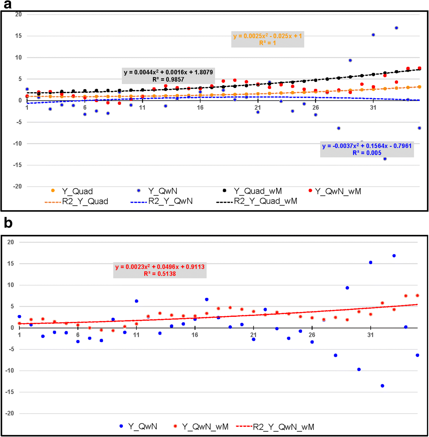
a Numerical experiment. An experimental realization: yQuad(orange; invariant), yQuad _ wM (black; invariant), YQwN (blue; variable), and YQwN _ wM(red; variable). Dashed lines indicate the second-order regressions and their coefficients of determination (R2). Note that physical units are dropped and axes kept dimensionless. Also note that now, in contrast to the example in Section 2.1, second-order regressions are appropriate as periodicity is omitted, and that here, the regression of YQuad _ wM falls above the regression of yQuad because we have not yet normalized the coefficients of YQuad _ wM, which steer the weight of memory over time. b Like a, but showing for a better overview only YQwN (blue; variable) and YQwN _ wM (red; variable) with its second-order regression (red solid line)
Supplementing Figs. 5 and 6: Compilation of regression parameters and coefficients of correlation, the latter between: (1) yQuad and yQuad _ wM (invariant); (2) yQuadand YQwN (variable); (3) YQwN _ wM and YQwN _ wM − 7yr (variable) with YQwN _ wM − 7yr being identical to YQwN _ wM but shifted backward in time (year 8 becomes year 1, year 9 year 2, and so on, while dropping the first 7 years of YQwN _ wM); and (4) yQuad and YQwN _ wM (variable). The first correlation coefficient indicates that limiting only the extent of memory back in time is not sufficient to overcome the “full memory” of yQuad. Correlation coefficients 2 and 3 seem to confirm that applying a high level of noise completely obliterates the second-order polynomial character of yQuad and that memory does not extend beyond 7 years. Finally, correlation coefficient 4 seems to confirm that memory (that is, YQwN _ wM) nullifies much of the obliteration brought about by YQwN
| Polynomial/regression for | a 2 | a 1 | a 0 | R 2 |
| y Quad | 0.0025 | − 0.0250 | 1.0000 | 1.000 |
| y Quad _ wM | 0.0044 | 0.0016 | 1.8079 | 0.9857 |
| Y QwN | − 0.0037 | 0.1564 | − 0.7961 | 0.005 |
| Y QwN _ wM | 0.0023 | 0.0496 | 0.9113 | 0.5138 |
| Y Lin, 7 yr | – | − 0.2434 | 2.1639 | 0.5142 |
| Y Lin _ exp , 7 yr | – | − 0.3966 | 2.9095 | 0.9049 |
| Coefficient of correlation between | ||||
| 1) yQuad & yQuad _ wM | Influence of memory (w/o noise) | 0.99 | ||
| 2) yQuad & YQwN | Influence of noise (obliteration) | 0.02 | ||
| 3) YQwN _ wM & YQwN _ wM − 7yr | Influence of memory after 7 years (w noise) | 0.06 | ||
| 4) yQuad & YQwN _ wM | Influence of memory in the presence of noise (reconstruction) | 0.71 | ||
YQwN _ wM overcomes much of that obliteration, bringing the curvature back to convex and increasing the R2 value substantially, here to greater than 0.5 (cf. also Table 3).
6.2 Part II: linear regression of the first seven points of y QwN _ wM

a Like Fig. 5a but additionally showing R1_Y_QwN_wM_hist_uw, a linear regression applying unit weighting [uw] back in time for the first seven points of YQwN _ wM(red; variable). The assumption here is that it is only these points (i.e., the extent of memory) of YQwN _ wM that observer O5 knows. For clarity, the legend specifies only items that are additional to those in Fig. 5a. b Like Fig. 5b but additionally showing R1_Y_QwN_wM_hist_ew, a linear regression applying exponential weighting [ew] back in time for the first seven points of YQwN _ wM, together with its in-sample [inConf] and out-of-sample [outConf] confidence bands. The borders of the confidence bands are indicated by upper [up] and lower [lo]. The assumption here is that observer O6 knows, like observer O5, only the first seven points (i.e., the extent of memory) of YQwN _ wM but, in addition, the weight of memory over time. For clarity, the legend specifies only items that are additional to those in Fig. 5b
By way of contrast, in deriving the linear regression in Fig. 6b the first seven points are weighted exponentially [ew] over time. Here, we assume that an observer (O6 hereafter) like observer O5, knows not only the first seven points (i.e., the extent of memory) of YQwN _ wM but also the weight of memory over time—an assumption that also requires discussion. The exponential weighting (the same as that underlying YQwN _ wM) results in a more confident linear regression called R1_Y_QwN_wM_hist_ew (in the figure) and YLin _ exp , 7yr (in Table 3) with an R2 value of about 0.90 and an even greater downward trend (− 0.40 versus − 0.24; cf. Table 3). Figure 6b also shows the confidence bands belonging to YLin _ exp , 7yr for the first 7 years [inConf] and beyond, the latter by means of the out-of-sample [outConf] continuation of the seven-year confidence band. As can be seen, YQwN _ wM crosses the 7-year confidence band from below to above and falls above the out-of-sample confidence band.
The reason for selecting this (unsuccessful), rather than another (successful) experimental realization is to prepare for the question as to whether we can make use of repeated regression analyses to capture the immediate future of YQwN _ wM? This will cause the experimental outlook to change from unsuccessful to promising.
Summary of results of 100 consecutive experiments where YQwN _ wM falls within the (in-sample and out-of-sample) confidence bands of YLin _ exp , 7yr for a time that corresponds to two times the extent of memory (= 14.5 years in the experiment). The individual experimental realizations are denoted by “1: YQwN _ wM in”; all others by “0: YQwN _ wM out”; indicating how often it is justified to shift the EO to today (here: year 7)
| Grouping of experiments | Coefficient of determination for | Coefficient of correlation for | No. of exp. | ||||
|---|---|---|---|---|---|---|---|
| Y Lin _ exp , 7 yr | Y Lin, 7 yr | Y QwN _ wM | yQuad & YQwN | YQwN _ wM & YQwN _ wM − 7yr | yQuad & YQwN _ wM | ||
| No grouping | 0.58 ± 0.32 | 0.50 ± 0.31 | 0.53 ± 0.22 | 0.10 ± 0.23 | 0.19 ± 0.35 | 0.62 ± 0.26 | 100 |
| \( 0:{Y}_{QwN\_ wM}\ out \) | 0.72 ± 0.26 | 0.60 ± 0.30 | 0.55 ± 0.22 | 0.15 ± 0.22 | 0.20 ± 0.37 | 0.65 ± 0.27 | 58 |
| \( 1:{Y}_{QwN\_ wM}\ in \) | 0.38 ± 0.30 | 0.35 ± 0.27 | 0.50 ± 0.21 | 0.03 ± 0.22 | 0.17 ± 0.32 | 0.59 ± 0.25 | 42 |
| 0 : YQwN _ wM out and R2 of YLin _ exp , 7yr > 0.30 | 0.77 ± 0.19 | 0.64 ± 0.28 | 0.56 ± 0.21 | 0.15 ± 0.21 | 0.19 ± 0.37 | 0.67 ± 0.24 | 53 |
| 1 : YQwN _ wM in and R2 of YLin _ exp < 0.70 | 0.27 ± 0.22 | 0.25 ± 0.19 | 0.50 ± 0.23 | 0.04 ± 0.23 | 0.19 ± 0.34 | 0.61 ± 0.25 | 34 |
| 0 : YQwN _ wM out and R2 of YLin _ exp , 7yr > 0.50 | 0.82 ± 0.13 | 0.68 ± 0.26 | 0.54 ± 0.21 | 0.13 ± 0.20 | 0.17 ± 0.36 | 0.66 ± 0.25 | 48 |
| 1 : YQwN _ wM in and R2 of YLin _ exp , 7yr < 0.50 | 0.18 ± 0.11 | 0.19 ± 0.15 | 0.50 ± 0.22 | 0.03 ± 0.23 | 0.18 ± 0.33 | 0.61 ± 0.26 | 27 |
In addition, Table 4 indicates that the obliteration of yQuad appears to be slightly greater on average for “1-experiments” than for “0-experiments” (cf. coefficients of correlation between yQuad and YQwN: 0.03 ± 0.23 versus 0.13 ± 0.20). However, it seems that “1-experiments” perform, on average, slightly better from a reconstruction perspective than “0-experiments.” In fact, they almost catch up (cf. coefficients of correlation between yQuad and YQwN _ wM: 0.61 ± 0.26 versus 0.66 ± 0.25).
In a nutshell, Table 4 confirms what common sense tells us: a world perceived too precisely is difficult to “project” even into the immediate future. Conversely, it is much easier to achieve if we are confronted with a highly imprecise world (forcing us to acknowledge our ignorance). This insight is not counter-intuitive but reflects prudent decision-making: In planning ahead, one is always well-advised to factor in some (not necessarily all) adverse effects that one can think of and that can easily occur. It is exactly this insight which tells us that (1) we should avoid following the footsteps of perfect forecasting to derive the EO of a data series (cf. Section 4) and (2) we can even derive a robust EO if we resist the temptation to describe the world we perceive too precisely.
7 Discussion
Our perspective piece in general and our numerical experiment in particular touch on a number of is sues the most pertinent of which we discuss below where we state what we know or believe we know and what we do not yet know.
Our approach of capturing memory is not restricted to identifying memory in time series of GHG emissions, in our case between emissions from newly installed furnaces (world without memory) and total emissions (world with memory). However, GHG emissions serve only as a case in point. Any two time series which are causally linked by memory (“memory-linked”) can be used instead, e.g., global GHG emissions and atmospheric concentrations or global mean surface temperature change.
We argue for and prefer using (at least, initially) synthetic data over real-world data. Synthetic data allow us to test the limits of deriving memory and the robustness of EOs by varying trend, periodicity, and stochastic remainder widely and in any combination.
In the numerical experiment in Sections 5 and 6, we assumed knowleged of the extent of memory in deriving a system’s EO. However, this piece of a priori information is not critical. According to our current understanding, the temporal extent of memory appears to be more important than both its weight (fading of memory) and quality (blurring of memory) back in time. From preliminary autocorrelation experiments, it appears that the extent of memory can be approximated even under unfavorable conditions. Our numerical experiment furthermore indicates that deriving an EO under unfavorable conditions is still possible too. However, the question of what constitutes favorable conditions needs to be explored thoroughly.
We assumed that we were able to repeat our numerical experiment multiple times, that is, that we would have available multiple realizations of a time series. But this does not disqualify us from using real-world data series which represent single realizations only. If applied in a piecemeal (learning and testing) mode, our method of deriving an EO is also applicable to analyzing real data series. However, the length of the data series relative to the extent of memory will affect the robustness of the EO. The main purpose of repeating experiments multiple times is to understand how long a data series needs to be to ensure robustness. Although we find that a system’s EO can be derived even under unfavorable conditions, we it is precisely for these reasons that we consider the time series used in the numerical experiment to be too short to determine the parameters of the underlying (here second-order) trend with high quality. That is, the insight that an EO can be derived under unfavorable conditions does not release us from an in-depth exploration of the issue of length of a data series vis-à-vis complexity of trend spotting.
But we see a trade-off evolving between the ignorance of understanding the past, e.g., by way of diagnostic modeling, and the robustness of the EO. Overestimating the precision of historical data may lead to an overly complex model for deriving an EO. This is problematic in two ways: First, it is known that over-parametrized diagnostic models are not necessarily optimal for use under prognostic conditions. Second, and of importance here, historical “surprises” (e.g., large outliers of random nature) are not treated as such; that is, the model tries to mimic them with the consequence that surprises are not expected to occur in the future. Adopting larger error margins for historical data while keeping model complexity to a minimum leads to a more stable trend and an EO sufficiently wide to allow for future surprises.
8 Summary and outlook
We opted for a perspective piece to discuss memory, persistence, and explainable outreach of forced systems, with GHG emissions into the atmosphere serving as our case in point. In the light of the continued increase in emissions globally vis-à-vis the reductions in them are required without further delay until 2050 and beyond, we conjecture that, being ignorant of memory and persistence, we may underestimate the “inertia” with which global GHG emissions will continue on their increasing path beyond today, which thus would also lead to overestimation of the amount of the reduction able to be achieved in the future. This issue is at the heart of mitigation and adaptation. For a practitioner, it translates to the problem of how persistently an emissions system behaves when subjected to a specified mitigation measure and what emissions level to adapt to for precautionary reasons in the presence of uncertainty.
We consider memory to be an intrinsic property of a system, retrospective in nature, and persistence to be a consequential (i.e., observable) feature of memory, prospective in nature and reflecting the tendency of a system to preserve a current state (including trend). Persistence depends on the system’s memory which, in turn, reflects how many historical states directly influence the current state. The nature of this influence can range from purely deterministic to purely stochastic.
Different approaches exist to capture memory. We capture memory generically with the help of three characteristics: its temporal extent and both its weight and quality over time. The extent of memory quantifies how many historical data directly influence the current data point. The weight of memory describes the strength of this influence (fading of memory), while the quality of memory steers how well we know the latter (blurring of memory). Capturing fading and blurring of memory in combination is novel.
In a numerical experiment with the focus on systemic insight, we cast a glance far ahead by illustrating one way to capture memory, and to understand how persistence plays out and how an EO can be derived even under unfavorable conditions. We discuss the experiment intensively with respect to how consequential it is, where it underperforms, and the research questions it provokes. However, the experiment does not exhibit fundamental shortfalls and does not restrict generalization.
- 1.
Do we have the right science in place to understand and treat memory appropriately?
- 2.
Given that memory links a system’s past with its near-term future and in the belief that knowing the system’s explainable outreach is of use for prognostic modelers and decision-makers, how well do we need to know the various characteristics of memory (e.g., those mentioned above), and can we differentiate and specify them by way of diagnostic data-processing alone, in order to delineate the system’s EO? Or, in other words, how much systems understanding do we need to have and to inject into the data-analysis process in order to enable such differentiation?
With regard to question 1, we demonstrate that treating memory appropriately requires its characteristics to be treated consistently for both the deterministic and the stochastic part of a time series, leading us onto new grounds to be mapped and explored, and multiple deterministic-stochastic approaches to be tested under controlled (i.e., lab) conditions initially and to be discussed widely—which is why we opt for a perspective piece before anything else. Any such approach falls in-between process-based modeling and time series analysis and contributes to closing the gap between the two.
With regard to question 2, we note that we study memory and persistence in a forward mode, and not yet in a backward mode; this means that we can contribute to this question only by way of initial insight. To this end, we can mention that we have reasons for optimism that the system’s EO can be derived under both incomplete knowledge of memory and imperfect understanding of how the system is forced. But we learn (1) that we should avoid following the footsteps of perfect forecasting to derive the EO of a data series; and (2) that we can derive a robust EO even if we resist the temptation to describe the world we perceive too precisely.
Determining the temporal extent of memory in the presence of (possibly great) noise is an important step, if not the most important. But we are interested in more, namely, how memory evolves back in time in terms of both weight and quality. That is, we are left with the challenge of acquiring a deeper systemic understanding to substantiate how memory plays out over time (exponentially, as in our numerical example, or otherwise). It remains to be seen whether meeting that challenge is feasible.
Although the prime intention of our perspective piece is to study memory, persistence, and explainable outreach of forced systems and, thus, to expand on the usefulness of GHG emission inventories, our insights indicate the high chance of our conjecture proving true: being ignorant of memory and persistence, we underestimate, probably considerably, the “inertia” with which global GHG emissions will continue on their historical path beyond today and thus we overestimate the amount of reductions that we might achieve in the future.
Notes
Acknowledgments
Open access funding provided by International Institute for Applied Systems Analysis (IIASA). The authors are grateful to IIASA and the Earth System Sciences Research Program of the Austrian Academy of Sciences to financing this research.
Acronyms and nomenclature
Aaperture (of the EO)
ARIMAautoregressive integrated moving average
ARFIMAautoregressive fractionally-integrated moving average
EMDempirical mode decomposition
EOexplainable outreach
ewexponential weighting
GHGgreenhouse gas
GOSATGreenhouse Gases Observing Satellite
IIASAInternational Institute for Applied Systems Analysis
inConfin-sample confidence band
IPCCIntergovernmental Panel on Climate Change
Llength (extent of EO)
lolower
Mmemory
O observer
OCO-2Orbiting Carbon Observatory-2
outConfout-of-sample confidence band
Rcoefficient of determination
SPMsummary for policymakers
ttime
UNFCCCUnited Nations Framework Convention on Climate Change
upupper
uwunit weighting
References
- Abarbanel HDI (2013) Predicting the future. Completing models of observed complex systems. Springer, New YorkGoogle Scholar
- Barkoulas JT, Baum CF (1996) Long-term dependence in stock returns. Econ Lett 53:253–259 http://citeseerx.ist.psu.edu/viewdoc/download?doi=10.1.1.470.3891&rep=rep1&type=pdf CrossRefGoogle Scholar
- Barros CP, Gil-Alana LA, Wanke P (2016) Brazilian airline industry: persistence and breaks. Int J Sustain Transp 10(9):794–804. https://doi.org/10.1080/15568318.2016.1150533 CrossRefGoogle Scholar
- Belbute JM, Pereira AM (2017) Do global CO2 emissions from fossil-fuel consumption exhibit long memory? A fractional integration analysis. Appl Econ 49(40):4055–4070. https://doi.org/10.1080/00036846.2016.1273508 CrossRefGoogle Scholar
- Caballero R, Jewson S, Brix A (2002) Long memory in surface air temperature: detection, modeling, and application to weather derivative valuation. Clim Res 21:127–140. https://doi.org/10.3354/cr021127 CrossRefGoogle Scholar
- Carbon Brief (2017) Analysis: Global CO2 emissions set to rise 2% in 2017 after three-year ‘plateau’. Carbon Brief, 13 November, London. https://www.carbonbrief.org/analysis-global-co2-emissions-set-to-rise-2-percent-in-2017-following-three-year-plateau (accessed 20 July 2018)
- Chow KV, Denning KC, Ferris S, Noronha G (1995) Long-term and short-term price memory in the stock market. Econ Lett 49:287–293. https://doi.org/10.1016/0165-1765(95)00690-H CrossRefGoogle Scholar
- Dajcman S (2012) Time-varying long-range dependence in stock market returns and financial market disruptions – a case of eight European countries. Appl Econ Lett 19(10):953–957. https://doi.org/10.1080/13504851.2011.608637 CrossRefGoogle Scholar
- Franzke C (2010) Long-range dependence and climate noise characteristics of Antarctic temperature data. J Clim 23(22):6074–6081. https://doi.org/10.1175/2010JCLI3654.1 CrossRefGoogle Scholar
- Hakkarainen J, Ialongo I, Tamminen J (2016) Direct space-based observations of anthropogenic CO2 emission areas from OCO-2. Geophys Res Lett 43:11400–11406. https://doi.org/10.1002/2016GL070885 CrossRefGoogle Scholar
- Hamal K (2010) Reporting GHG emissions: change in uncertainty and its relevance for the detection of emission changes. Interim Report IR-10-003, International Institute for Applied Systems Analysis, Laxenburg, Austria. http://pure.iiasa.ac.at/id/eprint/9476/1/IR-10-003.pdf
- Hansen PR, Lunde A (2014) Estimating the persistence and the autocorrelation function of a time series that is measured with error. Economet Theor 30(1):60–93. https://doi.org/10.1017/S0266466613000121 CrossRefGoogle Scholar
- IPCC (2001) In: Watson RT et al (eds) Climate Change 2001: Synthesis Report. A Contribution of Working groups I, II and III to the Third Assessment Report of the Intergovernmental Panel on Climate Change. Cambridge University Press, CambridgeGoogle Scholar
- Kantelhardt JW (2004) Fluktuationen in komplexen Systemen. Habilitationsschrift, Justus Liebig University Giessen. http://www.physik.uni-halle.de/Fachgruppen/kantel/habil.pdf
- Kantelhardt JW, Koscielny-Bunde E, Rybski D, Braun P, Bunde A, Havlin S (2006) Long-term persistence and multifractality of precipitation and river runoff records. J Geophys Res 111(D01106). https://doi.org/10.1029/2005JD005881
- Lennartz S, Bunde A (2009) Trend evaluation in records with long-term memory: application to global warming. Geophys Res Lett 36:L16706. https://doi.org/10.1029/2009GL039516 CrossRefGoogle Scholar
- Lennartz S, Bunde A (2011) Distribution of natural trends in long-term correlated records: a scaling approach. Phys Rev E 84:021129. https://doi.org/10.1103/PhysRevE.84.021129 CrossRefGoogle Scholar
- Lo AW (1991) Long-term memory in stock market prices. Econometrica 59(5):1279–1313 http://www.jstor.org/stable/2938368 CrossRefGoogle Scholar
- Lüdecke HJ, Hempelmann A, Weiss CO (2013) Multi-periodic climate dynamics: spectral analysis of long-term instrumental and proxy temperature records. Clim Past 9:447–452. https://doi.org/10.5194/cp-9-447-2013 CrossRefGoogle Scholar
- Majunmdar SN, Dhar D (2001) Persistence in a stationary time series. Phys Rev E 64:046123. https://doi.org/10.1103/PhysRevE.64.046123 CrossRefGoogle Scholar
- Marland G, Hamal K, Jonas M (2009) How uncertain are estimates of CO2 emissions? J Ind Ecol 13(1):4–7. https://doi.org/10.1111/j.1530-9290.2009.00108.x CrossRefGoogle Scholar
- Matsunaga T, Maksyutov S (eds) (2018) A guidebook on the use of satellite greenhouse gases observation data to evaluate and improve greenhouse gas emission inventories. Satellite Observation Center, National Institute for Environmental Studies, Japan http://www.nies.go.jp/soc/en/documents/guidebook/GHG_Satellite_Guidebook_1st_12b.pdf
- Mudelsee M (2014) Climate time series analysis. Classical statistical and bootstrap methods. Springer, ChamGoogle Scholar
- Oda T, Bun R, Kinakh V, Topylko P, Halushchak M, Lesiv M, Danylo O, Horabik-Pyzel J (2018) Assessing uncertainties associated with a high-resolution fossil fuel CO2 emission dataset: a case study for the ODIAC emissions over Poland. Mitig Adapt Strateg Glob Change (this special issue)Google Scholar
- Palma W (2007) Long-memory time series. Theory and methods. Wiley, HobokenCrossRefGoogle Scholar
- Solomon S, Daniel JS, Sanford TJ, Murphy DM, Plattner G-K, Knutti R, Friedlingstein P (2010) Persistence of climate changes due to a range of greenhouse gases. PNAS 107(43):18354–18359. https://doi.org/10.1073/pnas.1006282107 CrossRefGoogle Scholar
- UNFCCC (2018) Reporting requirements. United Nations Framework Convention on Climate Change, Bonn. https://unfccc.int/process/transparency-and-reporting/reporting-and-review-under-the-convention/greenhouse-gas-inventories-annex-i-parties/reporting-requirements (accessed 20 July 2018)
- Wu Z, Huang NE, Long SR, Peng C-K (2007) On the trend, detrending, and variability of nonlinear and nonstationary time series. PNAS 104(38):14889–14894. https://doi.org/10.1073/pnas.0701020104 CrossRefGoogle Scholar
Copyright information
Open Access This article is distributed under the terms of the Creative Commons Attribution 4.0 International License (http://creativecommons.org/licenses/by/4.0/), which permits unrestricted use, distribution, and reproduction in any medium, provided you give appropriate credit to the original author(s) and the source, provide a link to the Creative Commons license, and indicate if changes were made.